Fubini's Theorem Lesson

thingiverse

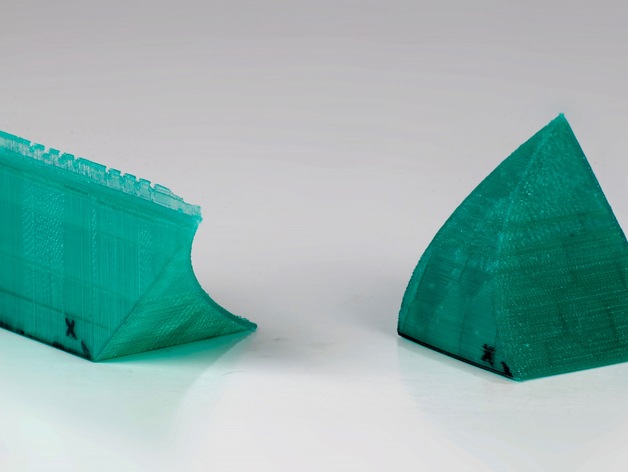
These two solid figures, Region E and Region F, are meant to be part of a multivariable calculus lesson on solid regions in three dimensions and Fubini's Theorem and Cavalieri's Principle. Students are given the two sets of inequalities below, and must first identify which model corresponds to which set of inequalities. Inequalities 1       Inequalities 2 0 < x < 1-z 0 < x < z+1 z^2 < y < 1 0 < y < (z-1)^2 0 < z 0 < z Students then use calculus to compare the volumes of the two models. This page is meant to complement the paper "3D Printed Manipulatives in a Multivariable Calculus Classroom" which will appear in PRIMUS. How I Designed This I used Mathematica's RegionPlot3D function to design these models. Specifically, for the first set of inequalities, RegionPlot3D[ x = z^2, {x, 0, 1}, {y, 0, 1}, {z, 0, 1}, BoxRatios -> Automatic, AxesLabel -> Automatic, PlotPoints -> 100 ] For the second set of inequalities, I used RegionPlot3D[ x Automatic, PlotPoints -> 100 ] These generated the following solid regions in Mathematica, which were exported to STL files using the Export function. I scaled the figures so that the unit length was 3 inches. Project: Solid Regions and Fubini's Theorem Overview & Background One of the major themes in multivariable calculus is finding the volume of solid regions in three dimensions. In order to get started on this topic, we need to establish a language for describing three-dimensional figures. One way to do this is to use inequalities in the three coordinate variables x, y, and z. The first part of this lesson gives students some practice with interpreting a set of inequalities as a descritption of a solid region. To start with volume calculations, students use Fubini's Theorem, tells us that the volume of a solid is equal to the definite integral of the cross-sectional area function. In other words, we can imagine cutting each figure into thin slices, multiplying the cross-sectional area of each slice by the thickness (estimating the volume of each slice), and then adding up the results to estimate the total volume. The thinner the slices, the better the estimate, and in the limit (with "infinitely thin" slices), we get the exact volume. This process is also known as Cavalieri's Principle. Lesson This lesson is best conducted in groups of two to four students. I printed a copy of each model for every group, and I drew coordinate axes on the models with a Sharpie. Once groups were decided, each group was given the labelled models of Region E and Region F, and told to answer the following questions. Below are two sets of inequalities. Which set of inequalities corresponds to Region E, and which corresponds to Region F? Give reasons for your answer. Inequalities 1       Inequalities 2 0 < x < 1-z 0 < x < z+1 z^2 < y < 1 0 < y < (z-1)^2 0 < z 0 < z Sketch cross-sections of each solid region taken parallel to the xy-plane. What shape are the cross-sections? Find the areas of the cross-sections as functions of z. Which region has a larger volume, E or F? Explain your answer in a few sentences. Preparation It is important that every student has a chance to handle the models, so I made sure to print enough copies of the modes ahead of time. I also think it was helpful to draw coordinate axes directly onto the models so that students could orient them correctly. As a warm-up to this activity, I had students deal with a simpler set of inequalities. In particular, I asked them to take 10 minutes at the beginning of class to build out of Play-Doh the region described by: 0 < x < 1 0 < y < 1 0 < z < x+y I found that this primed students with some strategies for thinking about how inequalities relate to solid regions.